Flow Maps and Distillation

The proliferation of Flow Maps and MeanFlow variant methods replacing diffusion and flow matching methods predicting instantaneous velocity for reduced sampling steps during inference. While Flow Maps have seen great improvements, still distribution matching techniques from an external model (teacher, adversarial) has its strengths and complements.

Here recent family of Mean Flow methods are covered along with the classic Score Distillation, Adversarial Distillation, and Consistency Distillation techniques together. Finally recent notable Flow Map techniques addressing different challenges (data free distillation, meta framework), alternative approaches to MeanFlow (TVM) and applications (video diffusion, riemmanian manifold) are addressed.

Foundations
MeanFlow Family
Score Distillation
Adversarial Distillation

Recent Flow Maps

1. Foundations

1.1 Diffusion

Diffusion models define a forward noising process that gradually corrupts data into noise, and a reverse process that learns to reconstruct data from noise. The main reason diffusion models became dominant is that they are stable and high-quality, but the tradeoff is slow iterative sampling.

1.1.1 Forward process (discrete DDPM view)

In DDPM, the forward process is a Markov chain:

\[q(x_t \mid x_{t-1}) = \mathcal{N}\!\left(\sqrt{1-\beta_t}\,x_{t-1}, \beta_t I\right),\]

where $\beta_t \in (0,1)$ is a variance schedule.

A key closed form is:

\[q(x_t \mid x_0) = \mathcal{N}\!\left(\sqrt{\bar\alpha_t}\,x_0,\,(1-\bar\alpha_t)I\right),\]

with

\[\alpha_t = 1-\beta_t,\qquad \bar\alpha_t=\prod_{s=1}^t \alpha_s.\]

So we can sample $x_t$ directly as:

\[x_t = \sqrt{\bar\alpha_t}\,x_0 + \sqrt{1-\bar\alpha_t}\,\epsilon,\qquad \epsilon \sim \mathcal{N}(0,I).\]

This is the standard “data + Gaussian noise” interpolation used in many diffusion derivations.

1.1.2 Reverse process and denoising objective

The generative model learns the reverse transitions

\[p_\theta(x_{t-1}\mid x_t),\]

which are parameterized via a neural network (predicting noise, $x_0$, or velocity depending on parameterization).

The most common training objective is noise prediction:

\[\mathcal{L}_{\text{simple}}(\theta) = \mathbb{E}_{t,x_0,\epsilon} \left[ \left\|\epsilon - \epsilon_\theta(x_t,t)\right\|^2 \right].\]

This objective is simple and works extremely well, but inference still requires many reverse denoising steps.

1.1.3 Continuous-time diffusion (SDE view)

A continuous-time diffusion can be written as an SDE:

\[dx = f(x,t)\,dt + g(t)\,dW_t,\]

where $f$ is drift, $g$ is diffusion scale, and $W_t$ is a Wiener process.

The reverse-time generative dynamics also form an SDE involving the score:

\[\nabla_x \log p_t(x).\]

This is the bridge to score-based generative modeling and continuous-time transport formulations.

1.1.4 Probability flow ODE (deterministic counterpart)

Every diffusion SDE has an associated deterministic probability flow ODE that shares the same marginals $p_t$:

\[\frac{dx}{dt} = f(x,t) - \frac{1}{2}g(t)^2 \nabla_x \log p_t(x).\]

This is huge conceptually because it turns diffusion sampling into solving an ODE, which directly connects to:

continuous normalizing flows,
flow matching,
rectified flow,
and later flow-map distillation methods.

So diffusion is not just “denoising noise,” it is also a continuous transport process in disguise.

1.1.5 Why diffusion motivates distillation

Diffusion teachers are strong but slow because generation requires many function evaluations (NFEs). Distillation methods aim to compress this long trajectory into:

few-step samplers (e.g. 2–8 steps),
or even one-step generators,

while preserving the teacher’s learned transport geometry.

This is exactly why Chapter 1 naturally progresses from Diffusion $\to$ Flow Matching $\to$ Flow Maps / Consistency / Distillation.

1.2 Flow Matching

Flow Matching

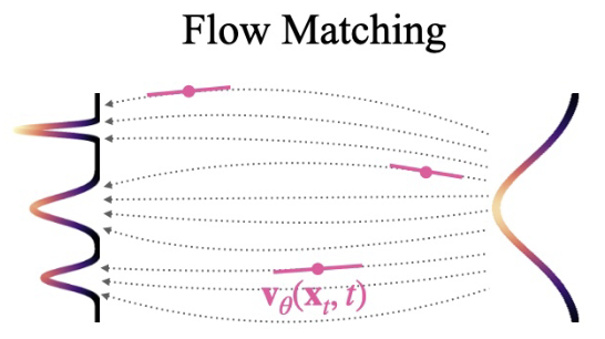
Figure 1. Flow Matching. from Sabour, Fidler, and Kreis (2025), Align Your Flow: Scaling Continuous-Time Flow Map Distillation (arXiv:2506.14603).

Flow Matching (FM) reframes generative modeling as directly learning a time-dependent velocity field that transports a simple source distribution (usually Gaussian noise) to the data distribution.

1.2.1 Core idea: learn the instantaneous velocity

Instead of learning reverse denoising conditionals, FM learns a vector field

\[u_\theta(x,t)\]

such that samples evolve via the ODE

\[\frac{dx}{dt} = u_\theta(x,t),\qquad t\in[0,1].\]

If this ODE is integrated from source noise at $t=0$ to $t=1$, the final samples should follow the data distribution.

1.2.2 Conditional path and target velocity

FM is usually trained by defining a conditional interpolation path between paired endpoints $(x_0,x_1)$:

\[x_t = \psi_t(x_0,x_1).\]

For simple linear interpolation:

\[x_t = (1-t)x_0 + tx_1.\]

The target velocity along this path is:

\[\dot{x}_t = \frac{d}{dt}\psi_t(x_0,x_1).\]

For the linear path, this becomes:

\[\dot{x}_t = x_1 - x_0.\]

The model is trained to match this conditional velocity in expectation:

\[\mathcal{L}_{\text{FM}}(\theta) = \mathbb{E}_{t,x_0,x_1} \left[ \left\|u_\theta(x_t,t)-\dot{x}_t\right\|^2 \right].\]

So FM is “supervised vector field learning” on a chosen path family.

1.2.3 Why FM is attractive

Compared to score/diffusion training, FM gives a very clean ODE-learning objective and avoids explicit score estimation. It is especially natural when you want to reason about:

transport geometry,
ODE trajectories,
and later finite-time maps (flow maps).

1.2.4 Limitation: local field, expensive sampling

FM learns a local tangent $u_\theta(x,t)$, not a finite-time jump. That means sampling still requires numerical integration:

\[x_{t+\Delta t} \approx x_t + \Delta t\,u_\theta(x_t,t)\]

(or higher-order solvers like Heun).

If trajectories are curved, discretization error accumulates, so many NFEs are needed. This is the main bottleneck that motivates:

Rectified Flow (straighter trajectories),
Flow Maps (direct time-to-time transport),
and distillation methods (few-step or one-step generation).

1.3 Rectified Flow

Rectified Flow (RF) keeps the ODE/transport framing of FM, but explicitly pushes the learned trajectories to become straighter, which makes them much easier to sample with few steps.

1.3.1 Motivation: straight trajectories are cheap

If a trajectory is highly curved, Euler updates need many small steps. If a trajectory is nearly straight, even a coarse solver can track it accurately.

So RF is basically a geometry-aware fix to the FM sampling bottleneck.

1.3.2 Linear interpolation path and velocity target

A standard RF path is the same linear interpolation:

\[x_t = (1-t)x_0 + tx_1,\]

with instantaneous derivative

\[\frac{dx_t}{dt} = x_1 - x_0.\]

RF trains a velocity field to match this transport direction along the path:

\[v_\theta(x_t,t) \approx x_1 - x_0.\]

A common training objective is:

\[\mathcal{L}_{\text{RF}}(\theta) = \mathbb{E}_{t,x_0,x_1} \left[ \left\|v_\theta(x_t,t)-(x_1-x_0)\right\|^2 \right].\]

This looks similar to FM, but the interpretation is sharper: RF cares about learning a transport field whose induced trajectories are easy to discretize.

1.3.3 Reflow (iterative rectification)

A major practical idea in RF is reflow:

Train an initial transport field.
Sample trajectories from the model.
Use those trajectories (or endpoint couplings) to retrain a straighter field.
Repeat.

Each round reduces curvature and improves few-step generation. This is why RF is often viewed as a bridge between classical diffusion/FM and modern one-step distillation.

1.3.4 Why RF matters

RF is the clean conceptual bridge to flow-map methods because it shifts the focus from “match local field” to “shape trajectories for fast transport.” Once you think this way, the next obvious step is:

Why learn only the local tangent at all?
Why not learn the finite-time map directly?

That is exactly the flow-map perspective.

1.4 Flow Map

Flow Map

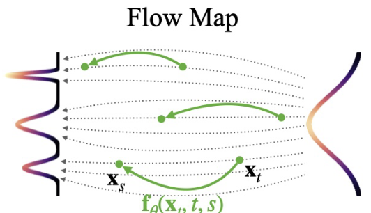
Figure 2. Flow Map. from Sabour, Fidler, and Kreis (2025), Align Your Flow: Scaling Continuous-Time Flow Map Distillation (arXiv:2506.14603).

Flow-map methods move beyond local vector fields and directly learn a time-to-time transport operator.

1.4.1 From vector field to finite-time map

Given a velocity field $u(x,t)$ and its ODE

\[\frac{dx}{dt}=u(x,t),\]

the associated flow map $\phi_u$ sends a state from time $t$ to time $s$:

\[\phi_u(x_t,t,s)=x_s.\]

So instead of learning only the local tangent $u(x,t)$, we learn the finite-time update:

\[x_s \approx \phi_\theta(x_t,t,s).\]

This is much more aligned with few-step sampling, because a single model evaluation can move across a large time interval.

1.4.2 Why flow maps help distillation

A flow field gives infinitesimal updates; a flow map gives finite jumps.

That means flow maps are naturally suited for:

few-step sampling (large $t\to s$ jumps),
teacher-student distillation (student imitates teacher transitions),
self-distillation (model supervises its own multistep consistency),
and data-free distillation variants (matching dynamics without original data).

This is the key conceptual move behind MeanFlow-family and FreeFlowMap-family methods.

1.4.3 Semigroup / composition structure

Exact flow maps satisfy a composition rule (semigroup property):

\[\phi(x_t,t,r) = \phi\!\left(\phi(x_t,t,s),\,s,\,r\right) \qquad \text{for } t \le s \le r.\]

This property is incredibly important because it gives a built-in consistency constraint across time triples. Many modern distillation methods exploit some version of this:

explicit composition matching,
consistency losses,
JVP-based local constraints that imply finite-time consistency.

1.4.4 Relation to FM and RF

FM learns $u(x,t)$ (local instantaneous velocity)
RF improves trajectory geometry (straighter ODE paths)
Flow Map learns $\phi(x_t,t,s)$ (finite-time transport)

So flow maps are not a totally different universe; they are the natural next abstraction after FM/RF if your goal is fast generation.

1.5 Consistency Models

Consistency Models (CMs) attack the same bottleneck from another angle: instead of learning a vector field or even an explicit flow map, they learn a cross-time consistent predictor that maps noisy states to a shared target representation (often an estimate of clean data).

This makes them one of the foundational one-step / few-step distillation paradigms.

1.5.1 Core consistency idea

Suppose $x_t$ and $x_s$ lie on the same teacher trajectory (or same underlying denoising path). A consistency model $f_\theta$ is trained so that: $f_\theta(x_t,t) \approx f_\theta(x_s,s),$ after the appropriate scaling/parameterization.

In words: different noise levels along the same trajectory should produce the same final prediction.

This is a cross-time agreement constraint, not just a local derivative-matching objective.

1.5.2 Why this enables one-step generation

Because the model is trained to collapse trajectory points to a common target, we can often sample by evaluating the model once (or very few times) from a noisy input.

This directly targets inference speed, unlike standard diffusion training which optimizes denoising accuracy at every step but does not inherently optimize for low-NFE sampling.

1.5.3 Teacher-student consistency distillation

A common setup is:

Start with a strong diffusion/score teacher.
Generate paired states $(x_t, x_s)$ on teacher trajectories.
Train the student consistency model to agree across those states.

This makes consistency models a very important predecessor to later:

flow-map distillation,
self-distillation,
and JVP-based transport-map objectives.

1.5.4 Conceptual relation to flow maps

Consistency models and flow-map methods are closely related in spirit:

Flow map view: learn explicit transport $\phi(x_t,t,s)$
Consistency view: learn a representation/prediction that is invariant (or aligned) across times on the same trajectory

Both replace purely local supervision with cross-time structure, which is exactly what you need for few-step and one-step generation.

2. MeanFlow Family

2.1 MeanFlow

2.1.1 Average velocity instead of instantaneous velocity

Mean Flow

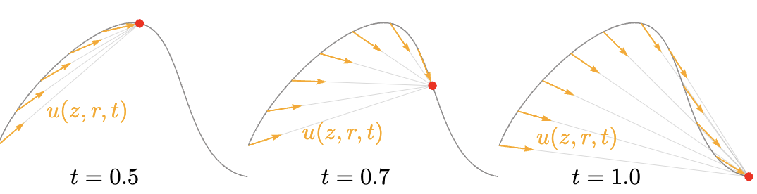
Figure 3. Mean Flow, with different target timestep $t$. from Geng et al. (2025), Mean Flows for One-step Generative Modeling (arXiv:2505.13447).

MeanFlow defines an average velocity

\[u(z_t, r, t)\]

over the interval $[r,t]$, so the displacement is:

\[(t-r)u(z_t,r,t).\]

2.1.2 The MeanFlow Identity (the central derivation)

Start from the definition:

\[(t-r)u(z_t,r,t) = \int_r^t v(z_\tau,\tau)\, d\tau\]

Differentiate both sides with respect to (t) (holding (r) fixed). By product rule + FTC:

\[u(z_t,r,t) + (t-r)\frac{d}{dt}u(z_t,r,t) = v(z_t,t)\]

Rearranging leads to the MeanFlow Identity:

\[u(z_t,r,t) = v(z_t,t) - (t-r)\frac{d}{dt}u(z_t,r,t)\]

2.1.3 Main Points

The authors rewrite an intractable target (the average velocity integral) into a trainable target:
- By first taking the derivative of both sides.
- Instantaneous velocity $v$ is available from FM-style interpolation.
- Total derivative term computed via JVP.
No explicit consistency regularizer is imposed.
The consistency-like structure falls out from the definition of average velocity.

2.1.4 MeanFlow loss

Parameterize $u_\theta(z_t,r,t)$, and regress to the identity-induced target:

\[\mathcal{L}_{\text{MeanFlow}}(\theta) = \mathbb{E}\left[ \left\| u_\theta(z_t,r,t) - \operatorname{sg}(u_{\text{tgt}}) \right\|_2^2 \right]\]

with

\[u_{\text{tgt}} = v_t - (t-r)\left(v_t \,\partial_z u_\theta + \partial_t u_\theta\right)\]

where the total derivative is implemented through a JVP along tangent $(v_t, 0, 1)$.

2.1.5 Sampling

Once you learn the average velocity, sampling is:

\[z_r = z_t - (t-r)u(z_t,r,t)\]

For 1-step:

\[z_0 = z_1 - u(z_1,0,1),\quad z_1 \sim p_{\text{prior}}\]

2.2 Improved MeanFlow (iMF)

iMF addresses two practical issues in MeanFlow:

the self-referential target,
fixed-CFG training (bad for inference-time flexibility).

2.2.1 MeanFlow as a v-loss

iMF rewrites the MeanFlow identity into a velocity regression form:

\[v(z_t) = u(z_t,r,t) + (t-r)\frac{d}{dt}u(z_t,r,t).\]

Then parameterize the RHS with $u_\theta$:

\[V_\theta = u_\theta(z_t,r,t) + (t-r)\,\mathrm{JVP}_{\mathrm{sg}}(u_\theta; v_\theta),\]

and train with a Flow-Matching-like loss

\[\mathcal{L}_{\mathrm{iMF}} = \mathbb{E}\left[\left\|V_\theta - (\epsilon-x)\right\|_2^2\right].\]

This is cleaner because the regression target is now the standard FM target $(\epsilon-x)$ rather than an apparent target constructed from $u_\theta$.

2.2.2 Flexible CFG as conditioning

Original MeanFlow supports CFG in 1-NFE, but with a fixed guidance scale chosen at training time.

iMF fixes this by making the guidance scale part of the conditioning:

guidance scale $\omega$ becomes an input condition,
the same model can be sampled with different CFG scales at inference.

That is a big deal because the optimal CFG scale shifts with model size, training progress, and NFE.

2.2.3 In-context conditioning

iMF also upgrades conditioning architecture:

conditions include $(r,t)$, class label $c$, and guidance-related variables $\Omega$,
each condition is represented with multiple learnable tokens,
all condition tokens are concatenated with image latent tokens and processed by the Transformer.

This allows:

support richer heterogeneous conditioning more naturally,
remove adaLN-zero,
cut params significantly (they report about 1/3 reduction in a base model setting).

2.3 AlphaFlow

AlphaFlow is the paper that gives the most useful conceptual interpretation of MeanFlow training.

2.3.1 Core insight: MeanFlow decomposes into two losses

AlphaFlow shows the MeanFlow objective can be algebraically decomposed into:

Trajectory Flow Matching (TFM)
Trajectory Consistency (TC)

The decomposition (up to a constant) is:

\[\mathcal{L}_{\mathrm{MF}} = \underbrace{\mathbb{E}\left[\|u_\theta(z_t,r,t)-v_t\|_2^2\right]}_{\mathcal{L}_{\mathrm{TFM}}} + \underbrace{\mathbb{E}\left[2(t-r)\,u_\theta^\top \frac{d u_\theta^-}{dt}\right]}_{\mathcal{L}_{\mathrm{TC}}} + C.\]

Interpretation:

TFM says “fit the trajectory-local velocity target.”
TC says “be self-consistent along the trajectory.”
MeanFlow is effectively a consistency-like model with extra trajectory FM supervision.

2.3.2 Why MeanFlow often needs lots of border-case FM samples

AlphaFlow also explains a weird empirical fact from MeanFlow:

MeanFlow works best when many samples use the border case $r=t$ (which looks like vanilla FM).

Their analysis shows this is not just a hack:

the gradients of TFM and trajectory consistency are often negatively correlated,
so the extra FM-style supervision helps stabilize and speed up training.

2.3.3 α-Flow loss: one objective that unifies TFM, Shortcut, MeanFlow

AlphaFlow defines a family of losses parameterized by $\alpha$:

\[\mathcal{L}_\alpha(\theta) = \mathbb{E}_{t,r,z_t} \left[ \alpha^{-1} \left\| u_\theta(z_t,r,t) - \left(\alpha \,\tilde v_{s,t} + (1-\alpha)\,u_{\theta^-}(z_s,r,s)\right) \right\|_2^2 \right],\]

where

\[s = \alpha r + (1-\alpha)t\]

is an intermediate time.

This unifies several training objectives:

$\alpha=1$ gives trajectory flow matching (with suitable $\tilde v_{s,t}$),
$\alpha=\tfrac{1}{2}$ recovers a Shortcut-style objective,
$\alpha \to 0$ recovers the MeanFlow gradient.

That is the key conceptual win: AlphaFlow puts FM, Shortcut, and MeanFlow on one continuum.

2.3.4 Curriculum

Because TFM and TC conflict early in training, AlphaFlow uses a curriculum:

start more FM-like (larger $\alpha$),
gradually anneal toward MeanFlow-like behavior (smaller $\alpha$).

This disentangles optimization and improves convergence.

2.3.5 Takeaways

AlphaFlow is best understood as:

a theory paper for MeanFlow optimization (decomposition + gradient conflict),
plus a practical training recipe (curriculum over $\alpha$) that improves one-step/few-step quality.

2.4 Accelerating and Improving MeanFlow

Understanding and Improving Mean Flow’s (UAIMF) main point is simple and very practical: MeanFlow training is bottlenecked by slow velocity formation and bad temporal-gap scheduling, so they speed up both. They propose two complementary components:

accelerate the velocity-learning part with standard diffusion training tricks (they use MinSNR or DTD), and
add a progressive weighting over the MeanFlow loss so the model learns small-gap average velocities first, then gradually expands to larger gaps.

2.4.1 Why MeanFlow trains slowly

UAIMF analyzes MeanFlow training through two coupled subproblems:

learning instantaneous velocity (the easier FM-like part),
learning average velocity over larger timestep gaps (the harder MeanFlow part).

Their empirical claim is that rapid velocity formation helps MeanFlow converge much faster, and that the temporal gap matters a lot: large-gap average-velocity learning is harder and should be delayed. This is why they combine velocity acceleration + progressive gap weighting.

2.4.2 Component 1: Accelerate the velocity part (MinSNR / DTD)

UAIMF tests one method from each category:

MinSNR as a loss-weighting acceleration method
DTD as a timestep-sampling acceleration method

and plugs them into MeanFlow training. They report both help, but emphasize that DTD is more robust across model scales because it changes the sampling distribution instead of interfering with MeanFlow’s own adaptive loss normalization.

2.4.3 Component 2: Progressive weighting on the MeanFlow loss

UAIMF progressively reweights the MeanFlow term so training starts by emphasizing small temporal gaps (easy) and gradually transitions to uniform weighting (full MeanFlow objective). Their weighting is:

\[\beta(\Delta t, s) = 1 - s + \lambda s (1 - \Delta t)\]

where:

$\Delta t$ is the temporal gap,
$s \in [0,1]$ is training progress,
$\lambda$ normalizes the expectation at initialization.

At initialization, the weighting prioritizes small gaps; by the end, it becomes uniform. They use a linear schedule by default:

\[s = 1 - \frac{i}{T}\]

and also discuss the generalized schedule:

\[s = 1 - \left(\frac{i}{T}\right)^k\]

with $k=1$ (linear) working best in their ablations.

2.4.4 Why the two components work together

Their ablation is clean:

velocity acceleration alone improves MeanFlow,
progressive $L_u$ weighting alone improves MeanFlow,
combining both works best.

They explicitly interpret this as:

acceleration methods quickly establish the instantaneous velocity foundation
progressive weighting improves average velocity learning over time

which is exactly the right mental model for MeanFlow optimization.

2.5 Decoupled MeanFlow

Decoupled MeanFlow is the strongest architectural update in this line. The core idea is: the encoder should care about the current timestep, and the decoder should care about the target timestep. They decouple timestep conditioning and turn a pretrained flow model into a flow-map model with almost no architectural surgery.

2.5.1 Core architectural idea: decouple encoder vs decoder conditioning

They reinterpret a flow model as:

\[v_\theta = g_\theta \circ f_\theta\]

with an encoder $f_\theta$ and decoder $g_\theta$. Then they argue the standard MeanFlow design is redundant because it feeds the next timestep $r$ everywhere. Their fix:

encoder gets current timestep $t$
decoder gets next timestep $r$

and the flow map becomes:

\[u_\theta(x_t, t, r) = g_\theta(f_\theta(x_t, t), r)\]

This is the defining DMF equation.

2.5.2 Why this matters: pretrained flow models already contain flow-map structure

DMF shows that a pretrained flow model can be converted into a flow map without fine-tuning, just by choosing an encoder/decoder split and decoding the representation with $r$. They report the converted DMF can even outperform the original flow model in some settings, which supports the claim that good flow-model representations are already enough for flow-map prediction.

This is a major conceptual shift: instead of training flow maps from scratch, you can reuse pretrained flow-model representations and repurpose the decoder.

2.5.3 Representation-first view

DMF explicitly argues that representation quality matters for flow maps. They show:

stronger pretrained encoders transfer better to flow-map fine-tuning
freezing encoder + tuning decoder already gives a large speed/quality gain
but true 1-step performance needs joint optimization (encoder cannot stay frozen forever)

This gives a practical recipe: pretrain a strong flow model first, then convert/fine-tune as DMF.

2.5.4 Training recipe: FM warm-up + MF fine-tuning

DMF also proposes a better training pipeline:

train a flow model with FM loss
convert to DMF
fine-tune with MeanFlow loss

They justify this on compute grounds (MF/JVP is expensive) and show it scales better than training a flow map from scratch. This is one of the most important practical contributions in the paper.

2.5.5 Enhanced training techniques

(a) Adaptive weighted Cauchy loss

They note MF loss has high variance, then replace the raw MSE-style MF loss with a Cauchy (Lorentzian) robust loss and an adaptive weighting term over timestep pairs. Their DMF objective is written as an adaptive weighted Cauchy form over the MeanFlow residual.

(b) Time proposal tailored to flow maps

They adapt timestep-pair sampling for flow maps (since you need ordered pairs with $t>r$). They sample two logit-normal values and sort them, and then bias the proposal toward larger gaps / smaller $r$ for better 1-step behavior, because converted DMF models are already strong near the diagonal $r \approx t$.

(c) Model Guidance (MG)

They use Model Guidance (MG) to avoid the full compute cost of CFG during training, and note MG is especially effective for training high-quality few-step flow maps. This is part of why their 1-step/4-step results are strong.

2.5.6 Takeaways

DMF is not just another MeanFlow variant. It reframes the problem:

MeanFlow gives the right objective (average velocity via JVP)
UAIMF / AlphaFlow improve optimization dynamics
DMF improves the architecture + training pipeline, and shows pretrained flow models are the best starting point

They report SOTA-level few-step results and show 1-step / 4-step generation approaching much more expensive flow-model sampling with large inference-speed gains.

3. Score Distillation

3.1 Variational Score Distillation (VSD)

3.1.1 Score Distillation Sampling (SDS)

VSD explicitly frames SDS as the starting point for text-to-3D optimization.
Given a differentiable renderer

\[g(\theta, c)\]

and a pretrained text-to-image diffusion model, SDS optimizes a single 3D parameter $\theta$ by minimizing a KL objective over noisy rendered images:

\[L_{\mathrm{SDS}}(\theta) := \mathbb{E}_{t,c} \left[ \frac{\sigma_t}{\alpha_t}\,\omega(t)\, D_{\mathrm{KL}} \big(q_t^\theta(x_t \mid c)\,\|\,p_t(x_t \mid y_c)\big) \right].\]

The practical gradient (the one everyone uses) is approximated as:

\[\nabla_\theta L_{\mathrm{SDS}}(\theta) \approx \mathbb{E}_{t,\epsilon,c} \left[ \omega(t)\big(\epsilon_{\mathrm{pretrain}}(x_t,t,y_c)-\epsilon\big) \frac{\partial g(\theta,c)}{\partial \theta} \right],\]

with

\[x_t = \alpha_t g(\theta,c) + \sigma_t \epsilon.\]

3.1.2 Why SDS is limited

SDS uses a single parameter $\theta$ and directly optimizes it, which makes it a mode-seeking procedure in practice.
VSD points out this is one reason SDS often gives over-smoothed / over-saturated / artifacted 3D results (especially in low-density regions of image space).

3.1.3 VSD: move from optimizing one 3D sample to learning a distribution over 3D parameters

The key VSD move is to define a distribution over 3D parameters

\[\mu(\theta \mid y)\]

instead of optimizing one fixed $\theta$.

Then VSD evolves particles by a Wasserstein gradient flow / particle ODE. The ODE uses a score difference between:

the score of noisy real images (from the pretrained diffusion model), and
the score of noisy rendered images (estimated by a learnable network).

The VSD particle dynamics are:

\[\frac{d\theta_\tau}{d\tau} = -\mathbb{E}_{t,\epsilon,c} \left[ \omega(t) \left( -\sigma_t \nabla_{x_t}\log p_t(x_t \mid y_c) - \big(-\sigma_t \nabla_{x_t}\log q_t^{\mu_\tau}(x_t \mid c,y)\big) \right) \frac{\partial g(\theta_\tau,c)}{\partial \theta_\tau} \right].\]

This is the conceptual heart of VSD:

teacher score pulls rendered images toward the text-conditioned image manifold,
rendered-image score corrects for the current particle distribution,
the difference gives a much better update than raw SDS.

3.1.4 The VSD score function estimator (this is the diffusion-distillation part)

VSD introduces a second noise predictor

\[\epsilon_\phi(x_t,t,c,y)\]

to estimate the score of noisy rendered images. It is trained with the standard diffusion noise-prediction objective on rendered images from the current particles:

\[\min_\phi \sum_{i=1}^n \mathbb{E}_{t,\epsilon,c} \left[ \left\| \epsilon_\phi\big(\alpha_t g(\theta^{(i)},c)+\sigma_t\epsilon,\ t,\ c,\ y\big)-\epsilon \right\|_2^2 \right].\]

This is the crucial diffusion-distillation component in VSD:

VSD distills a score model for the rendered-image distribution (not just the teacher),
then uses the difference of two scores for particle updates.

In practice, VSD parameterizes $\epsilon_\phi$ as either:

a small U-Net, or
a LoRA adaptation of the pretrained diffusion model (usually better fidelity).

3.1.5 VSD gradient used for updating the 3D particles

Once $\epsilon_\phi$ is trained, the per-particle VSD gradient becomes:

\[\nabla_\theta L_{\mathrm{VSD}}(\theta) = \mathbb{E}_{t,\epsilon,c} \left[ \omega(t)\, \big( \epsilon_{\mathrm{pretrain}}(x_t,t,y_c) - \epsilon_\phi(x_t,t,c,y) \big)\, \frac{\partial g(\theta,c)}{\partial \theta} \right],\]

with

\[x_t = \alpha_t g(\theta,c)+\sigma_t\epsilon.\]

This is the clean algorithmic form:

SDS uses $\epsilon_{\mathrm{pretrain}} - \epsilon$
VSD uses $\epsilon_{\mathrm{pretrain}} - \epsilon_\phi$

That replacement is the whole game.

3.1.6 VSD vs SDS

VSD shows SDS is a special case:

if you approximate the parameter distribution $\mu(\theta \mid y)$ by a single empirical point mass (one particle),
then the rendered-image score term degenerates to the sampled noise $\epsilon$,
and you recover vanilla SDS / SJC.

So the practical interpretation is:

SDS = single-point / no-generalization approximation
VSD = distributional score-distillation with a learned rendered-image score model

That is why VSD usually gives better diversity and better fidelity in text-to-3D than plain SDS.

3.2 DMD (Distribution Matching Distillation)

3.2.1 Core idea

DMD trains a one-step generator by taking a distribution-matching gradient (KL-driven, score-difference style). The distribution-matching improves realism and fixes pure regression collapse.

3.2.2 Distribution matching gradient

DMD computes a gradient by comparing two denoisers on the same noisy fake sample:

$\mu_{\text{real}}$: pretrained denoiser trained on real data
$\mu_{\text{fake}}$: denoiser trained on fake/generated data

For a fake image $x = G_\theta(z)$:

add random diffusion noise to get $x_t$
denoise with both networks
use the difference as the realism direction

The implementation-level gradient proxy is essentially:

\[\mathrm{grad} \propto \frac{ \mu_{\text{fake}}(x_t,t)-\mu_{\text{real}}(x_t,t) }{ \text{weighting\_factor} }\]

and they realize this as a stop-grad MSE objective on $x$ (so autograd yields the desired gradient direction).

This is the key DMD trick:

avoid backprop through a long teacher trajectory,
still get a distribution-level correction signal.

3.2.3 Practical read on DMD

DMD is strong because it is not just teacher regression:

the KL / distribution-matching gradient gives a realism signal beyond memorizing teacher trajectories,
the regression term keeps training stable.

That combo is why DMD was a big step for one-step image generation.

3.3 SiD (Score identity Distillation)

3.3.1 Core framing: explicit score matching on fake-data diffusion

SiD reframes one-step diffusion distillation as minimizing a score-difference loss on the diffused fake-data distribution.

Define the score difference:

\[\delta_{\phi,\theta}(x_t) := S_\phi(x_t) - \nabla_{x_t}\log p_\theta(x_t),\]

where:

$S_\phi(x_t)$ is the pretrained teacher score,
$p_\theta(x_t)$ is the diffused generator distribution.

Then SiD defines the theoretical objective (MESM / Fisher divergence):

\[L_\theta = \mathbb{E}_{x_t \sim p_\theta(x_t)} \left[ \|\delta_{\phi,\theta}(x_t)\|_2^2 \right].\]

This is the cleanest formulation in this chapter conceptually:

make the fake-data score match the teacher score.

3.3.2 Why SiD needs an auxiliary score network

The hard part is the generator score

\[\nabla_{x_t}\log p_\theta(x_t),\]

which is intractable directly.

SiD introduces a second network

\[f_\psi(x_t,t)\]

to approximate the conditional denoising mean / score-related quantity:

\[f_{\psi^*(\theta)}(x_t,t) = \mathbb{E}[x_g \mid x_t] = x_t + \sigma_t^2 \nabla_{x_t}\log p_\theta(x_t).\]

This gives a score-difference estimator:

\[\delta_{\phi,\psi^*(\theta)}(x_t) = \sigma_t^{-2}\big(f_\phi(x_t,t)-f_{\psi^*(\theta)}(x_t,t)\big).\]

So SiD turns score estimation into a diffusion-style denoising regression problem for $f_\psi$.

3.3.3 The naive approximation fails (important)

A very natural idea is to replace $\psi^*(\theta)$ with the current $\psi$ and use

\[\delta_{\phi,\psi}(x_t) = \sigma_t^{-2}\big(f_\phi(x_t,t)-f_\psi(x_t,t)\big),\]

then optimize the naive approximated loss

\[L_\theta^{(1)} = \mathbb{E}\left[\|\delta_{\phi,\psi}(x_t)\|_2^2\right].\]

SiD explicitly shows this can fail badly because:

the approximation error in $f_\psi$ enters the objective in a destabilizing way,
the loss depends on both score-estimation error and the true score difference.

This is the main reason SiD is not just “DMD but with a different notation.”

3.3.4 Projected score matching (SiD’s key fix)

SiD derives an alternative MESM form (Projected Score Matching) and then approximates it to get a much more stable objective:

\[L_\theta^{(2)} = \mathbb{E} \left[ \sigma_t^{-2}\, \delta_{\phi,\psi}(x_t)^\top \big(f_\phi(x_t,t)-x_g\big) \right].\]

This version is much more stable because it depends on the denoising residual

\[f_\phi(x_t,t)-x_g\]

instead of directly squaring the noisy score-difference estimate.

That is the algorithmic insight behind SiD:

use score identities to derive a loss that still targets MESM,
but behaves better under imperfect generator-score estimation.

3.3.5 Fused loss and alternating updates (the actual algorithm)

SiD trains with alternating updates:

Update $f_\psi$ (the generator-score estimator) with a diffusion / denoising loss.
Update $G_\theta$ using the SiD generator loss (built from the projected score-matching approximation / fused loss).

It also uses score gradients (backprop through both score networks), which distinguishes it from methods like Diff-Instruct and DMD.

In practice this is more memory/computation heavy, but it is a major reason SiD gets very strong one-step results.

4. Adversarial Distillation

4.1 Adversarial Diffusion Distillation (ADD)

ADD is the clean “diffusion-distill + GAN refine” recipe for turning a pre-trained diffusion teacher into a fast student (often 1-step or few-step), while explicitly preserving the teacher’s denoising behavior.

4.1.1 Core idea: combine adversarial learning with diffusion distillation

The student is trained with two losses:

Adversarial loss for photorealistic high-frequency detail
Diffusion distillation loss to stay aligned with the teacher’s denoising trajectory

The total generator objective is:

\[\mathcal{L}_G = \lambda_{\mathrm{adv}}\mathcal{L}_{\mathrm{adv}} + \lambda_{\mathrm{distill}}\mathcal{L}_{\mathrm{distill}}\]

This is the key point: ADD is not “just a GAN on top of diffusion outputs.” It is explicitly a teacher-constrained adversarial distillation method.

4.1.2 Adversarial part (generator + discriminator)

ADD uses a DINOv2-feature-based discriminator setup (projected / feature-space discrimination style), which is more stable and semantically informed than a plain pixel discriminator.

Generator adversarial loss (hinge-form style, on discriminator outputs) is:

\[\mathcal{L}_{\mathrm{adv}} = \mathbb{E}_{x_t, t, c}\left[D_\phi(\hat{x}_{\theta,t}, t, c)\right]\]

The discriminator is trained with a real/fake hinge objective plus regularization:

\[\mathcal{L}_D = \mathbb{E}_{x_t, t, c}\left[\max(0, 1 - D_\phi(\hat{x}_{\psi,t}, t, c))\right] + \mathbb{E}_{x_t, t, c}\left[\max(0, 1 + D_\phi(\hat{x}_{\theta,t}, t, c))\right] + \lambda_{R1}\mathcal{L}_{R1}\]

where:

$\hat{x}_{\psi,t}$ is the teacher-predicted denoised image
$\hat{x}_{\theta,t}$ is the student-predicted denoised image
the discriminator sees timestep and conditioning too, so the adversarial game is timestep-aware

4.1.3 Diffusion distillation part (the important anchor)

The distillation target is the teacher’s denoised estimate. ADD uses an SDS-style weighted regression to the teacher prediction:

\[\mathcal{L}_{\mathrm{distill}} = \mathbb{E}_{x_t,t,c}\left[ \omega(\lambda(t)) \left\| \hat{x}_{\theta,t} - \hat{x}_{\psi,t} \right\|_2^2 \right]\]

This is the “don’t drift too far from the teacher” term. Without it, pure adversarial training tends to hallucinate detail but break semantic / structural fidelity.

4.1.4 Why ADD matters

ADD became a strong template because it fixes the classic one-step problem:

pure distillation gives blurry or over-smoothed outputs
pure GAN gives sharp but unstable / off-manifold outputs

ADD gets both:

teacher alignment from diffusion distillation
sharpness and realism from adversarial training

4.1.5 Practical algorithm (high-level)

Sample $(x,c)$ and a timestep $t$
Corrupt to get $x_t$
Get teacher denoised prediction $\hat{x}_{\psi,t}$
Get student denoised prediction $\hat{x}_{\theta,t}$
Update discriminator with real = teacher prediction, fake = student prediction
Update student with:
- adversarial loss against discriminator
- weighted distillation loss to teacher prediction

4.2 LADD (Latent Adversarial Diffusion Distillation)

LADD is the latent-video extension of the adversarial distillation idea. The big shift is: do the adversarial game in latent/video space and train for long-horizon generation without requiring paired long targets.

4.2.1 Motivation: one-step video gets killed by exposure error

Teacher-forced diffusion distillation works okay for short clips, but for long autoregressive rollout:

errors accumulate
small distortions compound
teacher-forced supervision mismatches inference-time behavior

LADD’s fix is to lean harder into adversarial training and use the discriminator as the long-horizon supervision signal.

4.2.2 Key move: adversarial supervision replaces explicit per-step paired targets

Instead of requiring exact paired long-video targets (which are scarce and awkward), LADD trains the generator so each generated segment looks real to a discriminator.

That is the crucial algorithmic advantage:

supervised distillation needs paired targets and usually short clips
adversarial training only needs “real vs generated” segments

So LADD can train long-video generators from ordinary video data, even when very long continuous shots are rare.

4.2.3 Training pipeline structure (same spirit as APT/AAPT, but latent-video focused)

LADD-style training is best viewed as a staged pipeline:

Initialize from a pre-trained diffusion model
- keeps strong prior / semantics / motion prior
(Optional but common) distillation or adaptation warm-start
- stabilize the student before adversarial training
- preserve diffusion behavior early
Adversarial post-training in latent space
- discriminator distinguishes real vs generated latent video segments
- generator is trained autoregressively
- generated outputs are recycled as future inputs (student-forcing behavior)
Long-video segment training
- generate long sequences
- split into shorter overlapping segments for discriminator evaluation
- accumulate gradients segment-wise

This is the same deep idea that appears in modern real-time video papers: the discriminator gives a scalable supervision signal for long-horizon rollout.

4.2.4 Why latent adversarial training is stronger than pixel GAN in this setting

Doing the adversarial game in latent/video representation space helps because:

lower dimensionality → cheaper and more stable
closer to the model’s native generation space
easier to enforce temporal consistency than purely pixel GAN losses

In practice, this makes LADD-style methods much more compatible with:

one-step or few-step video generators
autoregressive rollout
KV-cache causal transformers

4.2.5 Main algorithmic takeaway

LADD is not just “ADD but for video.” It is the transition from:

paired denoising distillation to
distribution-level adversarial alignment for long-horizon latent rollout

That shift is what makes minute-long streaming generation feasible.

4.3 DiffRatio

DiffRatio is one of the most interesting adversarial/distillation hybrids because it gives a theory-backed correction to standard diffusion distillation.

4.3.1 Problem: teacher-forced distillation has a distribution mismatch

In teacher-forced distillation, the student is trained on teacher trajectories / noise states. But at inference, the student rolls out its own states.

So the student is optimized under the wrong state distribution.

This is the exact same failure mode as exposure bias in autoregressive models.

4.3.2 Density-ratio view (the core contribution)

DiffRatio frames this mismatch as a density ratio correction problem.

They derive a correction factor that reweights the distillation objective by a ratio between:

the student-induced trajectory distribution
the teacher/reference trajectory distribution

Conceptually:

\[\text{corrected objective} \;\sim\; \mathbb{E}_{\text{reference}} \left[ \frac{p_{\text{student}}}{p_{\text{reference}}} \cdot (\text{distillation error}) \right]\]

This is the main idea. The student should not just minimize teacher-forced error; it should minimize error under its own rollout distribution.

4.3.3 How they estimate the ratio (the adversarial/classifier trick)

The ratio is not known directly, so DiffRatio estimates it with a classifier (discriminator-like network).

Train a binary classifier to distinguish samples from:

teacher/reference distribution
student rollout distribution

Then convert the classifier logits into a density-ratio estimate. This is the same classic trick behind density-ratio estimation / f-GAN style estimation.

So the adversarial component is not only for realism here. It is used as a distribution correction estimator.

4.3.4 Final training recipe (algorithmically)

DiffRatio training has two coupled updates:

(A) Ratio estimator / classifier update

Train a classifier to separate:

reference (teacher) samples
student-generated samples

(B) Student update

Train the student with:

the original distillation loss
reweighted by the estimated density ratio

This directly targets the rollout mismatch that breaks one-step/few-step distillation.

4.3.5 Why this is important

DiffRatio is a more principled answer to the “teacher-student mismatch” than just adding more heuristics.

It says:

the issue is not only sharpness/blur
the issue is wrong training distribution
adversarial estimation can be used to fix the measure the student is trained under

That’s a very strong conceptual bridge between:

diffusion distillation
adversarial learning
off-policy / covariate-shift correction ideas

4.4 APT (and the modern AAPT extension)

APT (Adversarial Post-Training) is the core one-step video idea: start from a diffusion model, distill/adapt it, then use adversarial training to recover visual quality and speed.

AAPT extends APT to autoregressive real-time video generation with causal attention + KV cache.

4.4.1 The 3-stage training pipeline (the important part)

The modern APT/AAPT recipe is:

Diffusion adaptation
Consistency distillation
Adversarial training

This staged design is the key engineering insight. You do not jump directly from diffusion weights to GAN training.

Stage 1: Diffusion adaptation

Convert the pretrained video diffusion transformer into a causal/autoregressive architecture
Finetune with diffusion objective under teacher forcing
Preserve the diffusion prior while adapting architecture and inputs

Stage 2: Consistency distillation

Use consistency distillation as initialization before adversarial training
Speeds convergence and stabilizes the later adversarial phase
In AAPT, this is explicitly described as following APT

Stage 3: Adversarial post-training

Add a discriminator (initialized from diffusion weights in AAPT-style setups)
Train generator + discriminator adversarially
This improves frame quality and enables 1-step generation quality recovery

4.4.2 Why adversarial post-training is necessary after distillation

Consistency / diffusion distillation gets you speed, but often:

oversmooths details
weakens texture realism
accumulates errors in long rollout

Adversarial post-training fixes exactly that:

sharper details
better perceptual realism
stronger long-horizon behavior (especially with student-forcing)

This is why APT-style methods matter in practice: they are the bridge from “distilled but soft” to “distilled and actually usable.”

4.4.3 AAPT’s autoregressive extension (the useful algorithm detail)

AAPT extends APT in a way that is super relevant for streaming / interactive video:

Causal generator + KV cache

autoregressive frame generation
one latent frame per forward pass (1NFE)
reuse KV cache for speed

Student-forcing adversarial training

During adversarial training:

only the first frame is ground truth
afterward, the model feeds back its own generated frames
training behavior matches inference behavior

This is a big deal. It directly attacks exposure error instead of hiding it with teacher forcing.

4.4.4 Discriminator design and loss in the APT/AAPT line

AAPT uses:

a causal discriminator backbone (same family as the generator)
per-frame logits (not only clip-level), enabling parallel multi-duration discrimination
relativistic adversarial objective (R3GAN-style)
approximated R1/R2 regularization (following APT)

This is a very modern discriminator setup: it is designed for stability and long-video training, not old-school image GAN heuristics.

4.4.5 Long-video training trick (important)

AAPT-style training solves the long-video data problem by:

generating long videos
splitting them into short overlapping segments for discriminator evaluation
training the discriminator on real vs generated segments

This avoids needing rare long paired ground-truth targets and lets the generator learn long-horizon rollout behavior from ordinary video datasets.

That is the killer feature of adversarial post-training in this context: the discriminator supplies supervision at the distribution level, which scales to long sequences.

4.5 Comparisons

The adversarial line of diffusion distillation is not one thing; it has evolved through three distinct roles:

ADD: adversarial loss as a perceptual sharpness booster on top of diffusion distillation
APT / AAPT / LADD: adversarial post-training as the main way to make 1-step generators actually work for video and long-horizon rollout
DiffRatio: adversarial classifier as a density-ratio estimator for correcting teacher-student distribution mismatch

That progression is the real story: adversarial methods moved from “make it sharper” to “fix the training distribution and rollout behavior.”

5. FlowMap

5.1 Free FlowMap

Flow Map Distillation Without Data bias

5.1.1 Teacher-data mismatch (the hidden bug in many distillation pipelines)

Traditional flow-map distillation often samples intermediate states $x_t$ from an external dataset distribution and supervises the student using teacher velocities at those states.

But the student is supposed to reproduce the teacher’s sampling process, i.e. the trajectory distribution induced by the teacher from the prior.

Supervision states coming from a mismatched distribution results in a teacher-data mismatch:

the student is trained on states that are not on the teacher’s true rollout distribution,
more augmentation can worsen it,
student quality degrades.

This is a deep point because it says the standard “distill on data” recipe is fundamentally misaligned with the actual objective (imitate the teacher sampler).

5.1.2 Prior-only / self-generated flow-map objective

Supervise entirely from the prior and the student’s own generated states.

They derive a sufficient optimality condition leading to a loss of the form

\[\mathcal{L}_{\text{pred}} = \mathbb{E}_{z,\delta} \left[ \|F_\theta(z,\delta)-\operatorname{sg}(u_{\text{target}})\|^2 \right]\]

with

\[u_{\text{target}} = u(f_\theta(z,\delta),1-\delta) - \delta \,\partial_\delta F_\theta(z,\delta)\]

The key interpretation:

$f_\theta(z,\delta)$ defines the student’s current trajectory,
$\partial_\delta f_\theta$ is the student’s generating velocity,
the loss is equivalent to aligning the student generating velocity with the teacher field:

\[\partial_\delta f_\theta \approx u(f_\theta(z,\delta),1-\delta)\]

So the student learns to ride the teacher vector field along its own generated path, starting from pure noise, no dataset needed.

This is the right fix for teacher-data mismatch.

5.1.3 Gradient view

They explicitly write the optimization gradient in terms of a velocity mismatch

\[\Delta v_{G,u} = v_G - u\]

which is great because it makes gradient weighting / normalization tricks easier to reason about.

This is one of those “small” presentation choices that actually matters in practice.

5.1.4 Correction objective (fixing distribution drift, not just local velocity)

Here’s the catch: aligning generating velocity locally is necessary, but in finite-capacity/discrete training the generated distribution can still drift.

So they add a correction objective motivated from minimizing a KL term over intermediate marginals and then translating score mismatch into velocity mismatch (via the score–velocity equivalence for linear interpolants).

This yields a gradient proportional to

\[\nabla_\theta \; \mathbb{E}_{z,n,r} \left[ F_\theta(z,1)^\top \operatorname{sg} \left( v_N(I_r(f_\theta(z,1),n),r) - u(I_r(f_\theta(z,1),n),r) \right) \right]\]

where:

$u$ is the teacher marginal velocity,
$v_N$ is the student-induced noising marginal velocity,
$I_r(\cdot,\cdot)$ is the interpolation to intermediate time $r$.

Intuition:

the prediction loss aligns the student’s forward/generating flow
the correction loss aligns the student-induced noising marginals with the teacher’s marginals

That is a nice bidirectional correction mechanism.

5.2 Meta Flow Maps

Meta flow maps correspond to a stochastic flow map, which is important because deterministic flow maps are too rigid.

5.2.1 Why stochastic flow maps?

Deterministic flow-map learning works if the transport map is the right object. But for many diffusion-like processes, especially when you want richer uncertainty handling, a stochastic transition kernel

$\kappa_{t,s}(z_t, z_s)$ is the right object.

The paper frames this using:

marginal consistency
conditional consistency
a family of posterior conditionals $p_{1 t}$
and a diagonal supervision view

The important conceptual upgrade is:

instead of only learning deterministic trajectories,
learn a transition operator consistent with the stochastic process structure.

5.2.2 The diagonal condition (same role as FM diagonal supervision)

They derive that on the diagonal:

\[\kappa_{t,t}(z_t, z_1) = p_{1|t}(z_1 \mid z_t)\]

This is the stochastic analogue of “when $r=t$, your two-time object must match the one-time target.”

So the diagonal again plays the role of anchor supervision.

5.2.3 Pathwise/consistency relation for stochastic flow maps

They also derive a consistency/composition condition (their Eq. 23 in the snippet):

\[\kappa_{t,s}(z_t,z_s) = \mathbb{E}_{z_1 \sim p_{1|t}(\cdot|z_t)} \big[ \kappa_{u,s}(z_u,z_s) \big]\]

(with the appropriate latent dependence through $z_1$/paths)

The exact notation is heavier, but the key idea is the same as flow-map composition:

two-time transitions must compose correctly through intermediate times, but now in distributional form.

5.2.4 Their training objective (MFM loss)

They build:

a diagonal supervision loss (fit the posterior on diagonal time pairs),
a consistency loss (enforce off-diagonal composition consistency),
and combine them into an MFM objective:

\[\mathcal{L}_{\text{MFM}} = \mathcal{L}_{\text{diag}} + \lambda \mathcal{L}_{\text{cons}}\]

This is the stochastic counterpart of the deterministic progression:

diagonal target = “FM-like” anchor
off-diagonal consistency = “flow-map-like” propagation

5.2.5 Takeaways

This paper gives a more general lens:

MeanFlow / deterministic flow maps are one branch
stochastic transition learning is the broader object when uncertainty matters
the “diagonal + consistency” decomposition is the unifying pattern

This is exactly the kind of conceptual bridge diffusion researchers should care about.

5.3 Terminal Velocity Matching (TVM)

5.3.1 Core idea: match the terminal velocity of a learned flow map

TVM parameterizes a two-time displacement map (flow map increment) directly, instead of only learning the instantaneous velocity field.

Let the ground-truth displacement from time $t$ to $s$ be $f(x_t,t,s) := \psi(x_t,t,s) - x_t.$

TVM uses a model $f_\theta(x_t,t,s) = (s-t)F_\theta(x_t,t,s),$ and defines the model’s instantaneous velocity as the boundary derivative $u_\theta(x_t,t) := \left.\frac{d}{ds}f_\theta(x_t,t,s)\right|_{s=t} = F_\theta(x_t,t,t).$

This is the key unification:

the same network learns both
1. a large-step displacement map $f_\theta$, and
2. an infinitesimal velocity field $u_\theta$.

5.3.2 Why “terminal” velocity?

The ground-truth displacement satisfies $f(x_t,t,s)=\int_t^s u(x_r,r)\,dr.$

Differentiate w.r.t. the terminal time $s$: $\frac{d}{ds}f(x_t,t,s)=u(\psi(x_t,t,s),s).$

This is the terminal velocity condition.

The nice part is: if the terminal-velocity condition is satisfied along the trajectory, then the displacement map error is controlled (TVM shows an upper bound of displacement error by integrated terminal-velocity error). So instead of directly supervising the full ODE integral, TVM supervises the derivative at the terminal endpoint.

This is the conceptual contrast with MeanFlow:

MeanFlow differentiates w.r.t. the start time $t$,
TVM differentiates w.r.t. the end time $s$.

5.3.3 Proxy trick (how they make it trainable)

The terminal condition depends on unknown ground-truth objects:

$\psi(x_t,t,s)$ (true flow map)
$u(\cdot,s)$ (true velocity field)

TVM replaces them with model proxies: $u(\psi(x_t,t,s),s) \;\approx\; u_\theta\big(x_t + f_\theta(x_t,t,s),\, s\big).$

So the model predicts a displacement to a new point $x_s^{(\theta)} = x_t + f_\theta(x_t,t,s),$ then evaluates its own velocity field at that terminal point.

This makes the loss self-consistent and trainable in one stage.

5.3.4 TVM objective (the actual loss)

TVM jointly optimizes:

Terminal-velocity matching term (general $t \ge s$)
Flow Matching boundary term (special case / anchor)

Per-time objective: $\mathcal{L}_{\mathrm{TVM}}^{t,s}(\theta) = \mathbb{E} \Big[ \underbrace{ \left\| \frac{d}{ds}f_\theta(x_t,t,s) - u_\theta\big(x_t + f_\theta(x_t,t,s), s\big) \right\|_2^2 }_{\text{terminal velocity matching}} + \underbrace{ \|u_\theta(x_s,s)-v_s\|_2^2 }_{\text{Flow Matching anchor}} \Big].$

Where:

$x_s$ is sampled from the interpolation path (as in Flow Matching),
$v_s$ is the standard FM target velocity (e.g. for linear interpolation, $v_s = x_1 - x_0$).

Then the practical training objective is just expectation over sampled time pairs: $\mathcal{L}_{\mathrm{TVM}}(\theta) = \mathbb{E}_{t,s}\left[\mathcal{L}_{\mathrm{TVM}}^{t,s}(\theta)\right].$

5.3.5 EMA + stop-gradient version (important in practice)

Like consistency/distillation-style methods, TVM stabilizes training using:

EMA target network
stop-gradient on proxy paths

The practical version uses:

stop-grad copy for displacement branch,
stop-grad EMA copy for terminal velocity target.

Conceptually: $u_\theta\big(x_t + f_\theta(x_t,t,s),s\big) \;\to\; u_{\theta_{\text{EMA}}}^{\text{sg}} \Big(x_t + f_{\theta}^{\text{sg}}(x_t,t,s), s\Big).$

This avoids collapse / target chasing and makes the proxy supervision much more stable.

5.3.6 Why TVM is strong theoretically (the important claim)

TVM proves a distribution-level guarantee:

Under a Lipschitz assumption on $u_\theta(\cdot,s)$, a weighted time integral of the TVM objective upper-bounds the squared Wasserstein-2 distance between:

the model pushforward distribution (via the learned map), and
the true data distribution.

In spirit: $$ W_2^2(\text{model pushforward}, p_0) \;\lesssim\; \int_0^t \lambda(s)\,\mathcal{L}_{\mathrm{TVM}}^{t,s}(\theta)\,ds

C. $$

This is a big deal because many one/few-step distillation methods work well empirically but do not cleanly tie their loss to a distribution divergence.

5.3.7 Classifier-Free Guidance (CFG) version

TVM extends naturally to conditional generation with CFG.

They define a CFG-conditioned displacement map $f_\theta(x_t,t,s,c,w),$ where:

$c$ = class condition
$w$ = guidance scale

The practical CFG objective adds two important ideas:

Condition on $w$ directly
- The network sees the guidance scale at training time.
- This lets one model support multiple CFG scales.
Use a $1/w^2$ weighting
- Because target velocity magnitude scales roughly linearly with $w$,
- the loss can explode for large $w$ without correction.

So the conditional TVM loss is roughly: $\frac{1}{w^2} \left\| \frac{d}{ds}f_\theta(\cdot,c,w) - u_{\theta_{\text{EMA}}}^{\text{sg}}(\cdot,c,w) \right\|_2^2 + \mathcal{L}_{\mathrm{FM}}^{\text{CFG}}.$

This is one of the most practical contributions in the paper because it supports stable training under varying CFG.

5.3.8 Sampling algorithm

Once trained, sampling is dead simple and supports both 1-step and few-step generation without retraining.

For a sequence of times $1=t_0 > t_1 > \cdots > t_n=0,$ iterate: $x_{t_{k+1}} = x_{t_k} + f_\theta(x_{t_k}, t_k, t_{k+1}) = x_{t_k} + (t_{k+1}-t_k)F_\theta(x_{t_k}, t_k, t_{k+1}).$

So:

1-NFE: one direct jump $t=1 \to 0$
few-NFE: chain multiple learned jumps
no ODE solver needed (the network itself is the integrator)

This is exactly why flow-map-style methods are so appealing for distillation and fast sampling.

5.3.9 JVP term and implementation detail (important for “algorithm” understanding)

Because $f_\theta(x_t,t,s)=(s-t)F_\theta(x_t,t,s),$ the terminal derivative expands as $\frac{d}{ds}f_\theta(x_t,t,s) = F_\theta(x_t,t,s) + (s-t)\,\partial_s F_\theta(x_t,t,s).$

That second term is a Jacobian-vector product (JVP) through the network.

TVM’s practical novelty is not just using JVP, but supporting:

JVP through FlashAttention
backprop through the JVP result

That matters a lot for DiT-scale transformers, because naive PyTorch attention + JVP is too slow / memory-heavy.

5.3.10 Practical tricks that actually matter (from the paper)

TVM adds several engineering choices that are unusually important:

Semi-Lipschitz control in DiT
- The theory needs Lipschitzness-ish behavior.
- Vanilla DiT components (LayerNorm/SDPA) are problematic.
- They replace key normalizations with RMSNorm-style variants and normalize AdaLN modulation terms.
AdamW $\beta_2 = 0.95$
- Higher-order gradients from JVP make training noisy.
- Lower $\beta_2$ stabilizes second-moment tracking.
Scaled parameterization for CFG
- Make the model output scale with $w$ by construction: $f_\theta(x_t,t,s,c,w)=(s-t)\,w\,F_\theta(x_t,t,s,c,w).$
- This improves optimization under large guidance.
Time sampling matters
- They ablate multiple $(t,s)$ sampling schemes.
- Biasing toward larger jumps (larger $t$, smaller $s$) helps, but too aggressive hurts.
- They also find using a separate time distribution for the FM anchor term can help.

3.3.11 TVM vs MeanFlow (the clean comparison)

MeanFlow

matches a derivative condition w.r.t. start time $t$
propagates $u(x_t,t)$ through the JVP path
more sensitive to random CFG because the velocity magnitude directly enters the JVP branch

TVM

matches a derivative condition w.r.t. terminal time $s$
JVP is w.r.t. $s$ (cleaner and more stable under random CFG)
has a clearer Wasserstein-style distribution guarantee
naturally supports one-step and few-step jumps with the same network

This is why TVM is a strong “algorithmic” evolution of flow-map distillation rather than just another loss tweak.

5.4 Transition Matching Distillation

Transition Matching Distillation (TMD) bridges engineering and theory based adaptation of MeanFlow to video distillation.

5.4.1 Core problem setup

They want to distill a pretrained video diffusion teacher into a faster student. Direct one-stage distillation is hard in video because:

the space is huge,
temporal consistency matters,
transformer-based video models make JVP painful (esp. attention kernels/FSDP/context parallelism).

So TMD uses two stages.

5.4.2 Stage 1: Transition Matching MeanFlow (TM-MF)

This is the key new idea.

Instead of applying MeanFlow directly in the original latent/data space, they define an inner transition problem and parameterize a conditional inner flow map via average velocity:

\[f_\theta(y_s,s,r;m) = y_s + (s-r)u_\theta(y_s,s,r;m)\]

where $m$ is a feature extracted from the main backbone.

Then they use a MeanFlow-style objective to train this transition head.

A very practical (and nontrivial) design choice:

they reparameterize the average velocity to stay aligned with the teacher head:

\[u_\theta(y_s,s,r;m) = y_1 - \text{head}_\theta(y_s,s,r;m)\]

This is not cosmetic. It keeps the new head close to teacher semantics, which improves stability.

5.4.3 JVP issue and finite-difference approximation

This paper is very realistic about systems constraints:

exact JVP is annoying with large-scale video transformer stacks (FlashAttention, FSDP, context parallelism),
so they use a finite-difference approximation of the JVP.

That’s a practical compromise:

theoretically less clean than exact JVP,
but massively easier to integrate into production-grade training code.

5.4.4 Stage 2: Distributional distillation objective

After TM-MF pretraining, they switch to a stronger distillation stage using a VSD/discriminator-style objective (their simplified algorithm shows):

\[\mathcal{L} = \text{VSD}(\hat{x}) + \lambda \cdot \text{Discriminator}(\hat{x})\]

So the conceptual split is:

Stage 1 (TM-MF): learn a good transition-aware student parameterization, bootstrap geometry/dynamics
Stage 2: sharpen sample quality and distribution match

This is a strong template for hard domains (video, 3D, multimodal) where pure one-shot distillation is brittle.

5.4.5 Why TMD is strong

TMD wins because it combines both worlds:

trajectory-based structure (TM-MF / flow-map adaptation)
distribution-based distillation (DMD2-v)

And it does so with an architecture that respects the hierarchical structure of big video diffusion Transformers.

That’s why it gets a better speed-quality tradeoff than plain one-step/few-step distillation baselines in video.

Flow Maps and Distillation

Table of Contents

1. Foundations

1.1 Diffusion

1.1.1 Forward process (discrete DDPM view)

1.1.2 Reverse process and denoising objective

1.1.3 Continuous-time diffusion (SDE view)

1.1.4 Probability flow ODE (deterministic counterpart)

1.1.5 Why diffusion motivates distillation

1.2 Flow Matching

1.2.1 Core idea: learn the instantaneous velocity

1.2.2 Conditional path and target velocity

1.2.3 Why FM is attractive

1.2.4 Limitation: local field, expensive sampling

1.3 Rectified Flow

1.3.1 Motivation: straight trajectories are cheap

1.3.2 Linear interpolation path and velocity target

1.3.3 Reflow (iterative rectification)

1.3.4 Why RF matters

1.4 Flow Map

1.4.1 From vector field to finite-time map

1.4.2 Why flow maps help distillation

1.4.3 Semigroup / composition structure

1.4.4 Relation to FM and RF

1.5 Consistency Models

1.5.1 Core consistency idea

1.5.2 Why this enables one-step generation

1.5.3 Teacher-student consistency distillation

1.5.4 Conceptual relation to flow maps

2. MeanFlow Family

2.1 MeanFlow

2.1.1 Average velocity instead of instantaneous velocity

2.1.2 The MeanFlow Identity (the central derivation)

2.1.3 Main Points

2.1.4 MeanFlow loss

2.1.5 Sampling

2.2 Improved MeanFlow (iMF)

2.2.1 MeanFlow as a v-loss

2.2.2 Flexible CFG as conditioning

2.2.3 In-context conditioning

2.3 AlphaFlow

2.3.1 Core insight: MeanFlow decomposes into two losses

2.3.2 Why MeanFlow often needs lots of border-case FM samples

2.3.3 α-Flow loss: one objective that unifies TFM, Shortcut, MeanFlow

2.3.4 Curriculum

2.3.5 Takeaways

2.4 Accelerating and Improving MeanFlow

2.4.1 Why MeanFlow trains slowly

2.4.2 Component 1: Accelerate the velocity part (MinSNR / DTD)

2.4.3 Component 2: Progressive weighting on the MeanFlow loss

2.4.4 Why the two components work together

2.5 Decoupled MeanFlow

2.5.1 Core architectural idea: decouple encoder vs decoder conditioning

2.5.2 Why this matters: pretrained flow models already contain flow-map structure

2.5.3 Representation-first view

2.5.4 Training recipe: FM warm-up + MF fine-tuning

2.5.5 Enhanced training techniques

(a) Adaptive weighted Cauchy loss

(b) Time proposal tailored to flow maps

(c) Model Guidance (MG)

2.5.6 Takeaways

3. Score Distillation

3.1 Variational Score Distillation (VSD)

3.1.1 Score Distillation Sampling (SDS)

3.1.2 Why SDS is limited

3.1.3 VSD: move from optimizing one 3D sample to learning a distribution over 3D parameters

3.1.4 The VSD score function estimator (this is the diffusion-distillation part)

3.1.5 VSD gradient used for updating the 3D particles

3.1.6 VSD vs SDS

3.2 DMD (Distribution Matching Distillation)

3.2.1 Core idea

3.2.2 Distribution matching gradient

3.2.3 Practical read on DMD

3.3 SiD (Score identity Distillation)

3.3.1 Core framing: explicit score matching on fake-data diffusion

3.3.2 Why SiD needs an auxiliary score network

3.3.3 The naive approximation fails (important)

3.3.4 Projected score matching (SiD’s key fix)

3.3.5 Fused loss and alternating updates (the actual algorithm)

4. Adversarial Distillation