Joint Reward Alignment and Distillation in Video Diffusion

Reinforcement learning and reward alignment post-training can benefit video diffusion models orthogonally from pre-training and step-distillation.

I implemented several approaches to video diffusion post-training in FastVideo. The progression was Flow-GRPO → DiffusionNFT → DMDR → finite-transition posterior alignment, followed by reward-based velocity matching (RVM) for H3.

Two problems emerge: improving generated videos according to a reward, and preserving quality when generation takes only a few steps. These are mostly addressed separately but I’ve been interested in approaches to unify and jointly optimize for both metrics.

These experiments explore where to apply the reward signal: stochastic transitions, the pretrained flow-matching objective, or the finite transitions a distilled model actually executes.

Below are the core objectives, the adaptations I made for video, and what the runs showed. The experiments used different models and budgets; they are a worklog, not a controlled ranking of all five methods. Code branches · Experiment slides.

Throughout, $x_0$ denotes a clean video latent, $\epsilon$ Gaussian noise, and $c$ a prompt. With the noise-at-one convention, ordinary flow matching uses

\[x_t=(1-t)x_0+t\epsilon,\qquad u=\epsilon-x_0,\qquad \mathcal L_{\mathrm{FM}}=\mathbb E\|v_\theta(x_t,t,c)-u\|^2.\]

1. Flow-GRPO: stochastic exploration for video

Flow-GRPO makes flow-model transitions stochastic so that they have tractable probabilities. For $K$ videos generated from the same prompt, define the relative advantage and transition likelihood ratio as

\[A_i=\frac{R_i-\bar R_c}{s_c+\varepsilon},\qquad \rho_{i,t}=\frac{p_\theta(x_{t-\Delta}^{(i)}\mid x_t^{(i)},c)} {p_{\mathrm{old}}(x_{t-\Delta}^{(i)}\mid x_t^{(i)},c)}.\]

The core update is the clipped policy-gradient loss:

\[\mathcal L_{\mathrm{GRPO}} =-\mathbb E_{i,t}\!\left[ \min\!\left(\rho_{i,t}A_i, \operatorname{clip}(\rho_{i,t},1-\delta,1+\delta)A_i\right) \right]+\lambda\mathcal L_{\mathrm{ref}}.\]

Here $\mathcal L_{\mathrm{ref}}$ is an optional KL penalty to a frozen reference. The strength is straightforward credit assignment from a black-box terminal reward, without training a value model. For video, the difficulty is the cost and variance of long rollouts.

Shared noise controls scene variation; independent SDE draws supply exploration. Terminal rewards train the stochastic decisions. Whole prompt groups are placed on one GPU.

What mattered in my implementation:

Flow-SDE rollouts with a stochastic window. Explore within a limited portion of the trajectory and use deterministic ODE steps elsewhere. The stochastic step has the form $x_{t-\Delta}=\mu_\theta(x_t,t)+\sigma_t\sqrt{\Delta}\,z$, with $z\sim\mathcal N(0,I)$. Its corrected drift and Gaussian noise give a transition whose log-probability can be recomputed during training.
Shared initial latents. Candidates for one prompt can share their starting noise while taking different stochastic steps. This reduces variation from unrelated initial scenes and makes reward comparisons more focused.
Keep whole prompt groups on one GPU/rank. The sampler assigns all $K$ candidates together, making each group’s reward statistics locally available. The checked-in trainer still gathers rewards for its advantage/statistics path, so group placement should not be confused with eliminating every collective.
Asynchronous scoring and reward-model offloading. Submit reward work while collecting subsequent samples, and move reward models off GPU when idle to free memory. Actual overlap depends on the scorer and available memory; offloading trades transfer time for capacity.

This worked reasonably well as a video RL baseline. The practical lesson was that controlling rollout variance and scheduling reward computation mattered as much as the policy loss. Implementation.

2. DiffusionNFT: reward learning in the forward process

DiffusionNFT is one of my favorites because it brings post-training back to the flow-matching formulation. Generate a video, score it, then re-noise its final latent to construct supervised training states. The optimizer needs endpoints, not reverse-trajectory likelihoods, so rollout sampling can use a different solver.

Let $\bar v$ be the detached old-model prediction and $0\le r\le1$ a clipped, rescaled reward advantage. NFT constructs positive and implicit-negative predictions:

\[v^+=\bar v+\beta(v_\theta-\bar v),\qquad v^-=\bar v-\beta(v_\theta-\bar v).\]

Writing $\ell(v)$ for the forward reconstruction loss, the objective has the form

\[\mathcal L_{\mathrm{NFT}} =\mathbb E\!\left[r\ell(v^+)+(1-r)\ell(v^-)\right] +\lambda\|v_\theta-v_{\mathrm{ref}}\|^2.\]

High-reward samples pull toward their reconstruction target; low-reward samples push in the opposite direction through $v^-$. This is BCE-like weighting of two reconstruction losses, not a literal binary-classifier loss. My implementation reconstructs $\hat x_0=x_t-tv$, uses detached error normalization, and includes overall loss scaling omitted above.

Using the pretrained prediction space and a reference anchor gives a natural way to limit drift from pretrained behavior. It also lets me use Flow-UniPC, a higher-order solver, without deriving its sampling likelihood.

DiffusionNFT scores generated endpoints, re-noises their latents, and forms positive and implicit-negative velocity predictions on opposite sides of the detached old prediction. Reward weights their reconstruction losses. — NFT separates rollout sampling from forward-process training. The two predictions reconstruct the same endpoint, with reward controlling their weights; no rollout likelihood is needed.

My video adaptations:

Replace the image-reward setup with VideoAlign: visual quality (VQ), motion quality (MQ), and text alignment (TA).
Gather prompt identities and rewards across GPUs before computing per-prompt advantages. Unlike the intact GRPO groups, NFT’s repeated prompts can span ranks; normalizing each fragment independently changes the learning signal.
Count timestep microsteps in gradient accumulation and flush leftover gradients at the end of the inner loop. Otherwise the optimizer cadence changes silently with the number of training timesteps.
Lower the video learning rate to $2\times10^{-6}$ in the checked-in recipe; use 50-step Flow-UniPC, flow shift 8, and CFG 6 for both rollout and validation. Solver-agnostic training does not mean CFG-free sampling is best for every video model. Recipe and code.

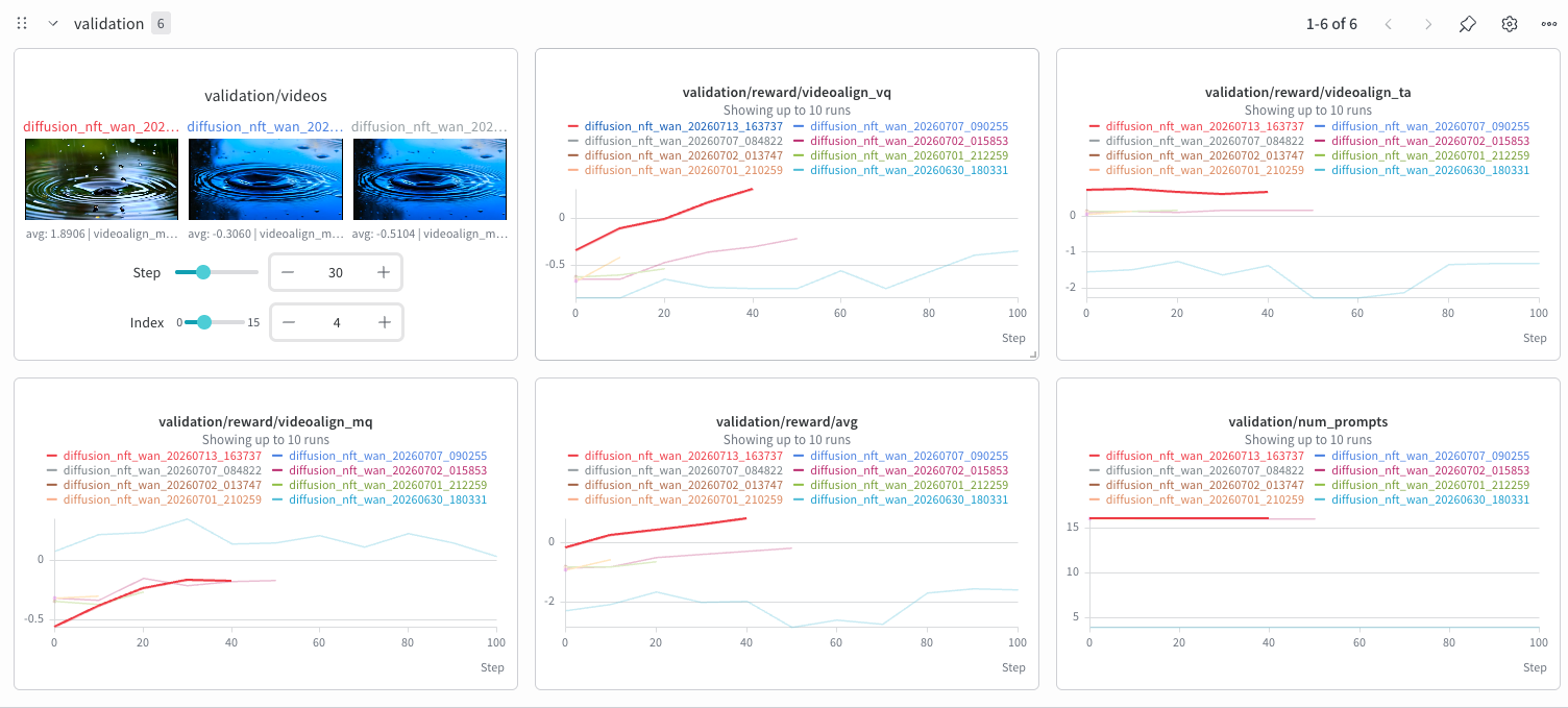
The W&B snapshot shows improving validation VQ and aggregate reward in the stronger NFT runs, with more modest MQ improvement and relatively flat TA. That was encouraging, although the small validation sets and differing configurations do not isolate which change caused the gain.

W&B DiffusionNFT validation charts showing visual quality, text alignment, motion quality, aggregate reward, and validation prompt counts across experimental runs. — NFT validation curves from the experiment slides. These are different run configurations, not a controlled solver or CFG ablation. Click to inspect the original chart.

3. DMDR: combining distillation and reward alignment

DMDR addresses the next problem: reward alignment should work while distilling a generator to fewer steps. Distribution matching supplies a teacher-based constraint, while reward optimization can move the student beyond simply copying the teacher.

I adapted it to video by replacing the original image-based reward/adversarial setup with NFT-style positive/negative learning from black-box video rewards. The student objective was

\[\mathcal L_{\mathrm{student}} =\lambda_R\mathcal L_{\mathrm{NFT,policy}} +\lambda_D\mathcal L_{\mathrm{DMD}} +\lambda_{\mathrm{ref}}\|v_\theta-v_{\mathrm{ref}}\|^2.\]

The DMD term re-noises the student’s predicted clean latent and compares a frozen teacher with a learned fake-score model. In the implementation, its correction is proportional to $\hat x_0^{\mathrm{fake}}-\hat x_0^{\mathrm{teacher}}$; a detached-target regression sends the student against that discrepancy. The critic learns separately by flow matching on student samples.

My DMDR adaptation combines black-box reward learning with teacher-based distribution matching. Both update the student; the fake-score critic learns separately on student samples.

The main training controls were a DMD-only cold start, more frequent critic updates than student updates, and time-dependent noise sampling and teacher guidance. For Wan, I used decaying teacher CFG in place of the reference implementation’s architecture-specific guidance hook. Video adaptation.

This was harder to train and worked less well in my runs. My suspicion is that simply adding reward and distribution-matching terms leaves their directions and scales poorly coordinated. That is a hypothesis, not an ablation result. It motivated a more direct question: can reward improve the exact transitions used by a few-step generator?

4. Finite-transition posterior projection alignment

I implemented this on the four-step AnyFlow-Wan model. Each update starts from a shared intermediate state, samples candidate next states from a local Gaussian policy, and completes each candidate with the deterministic suffix. Terminal video rewards therefore compare alternative decisions at the same transition.

The ideal local target is a reward-tilted behavior distribution:

\[q^*(a\mid s)\propto p_{\mathrm{old}}(a\mid s) \exp\!\left(R(y(a))/\tau\right).\]

Temperature $\tau$ controls reward selectivity. For $K$ sampled actions, the implemented centered projection update is

\[w_i=\frac{\exp(R_i/\tau)}{\sum_j\exp(R_j/\tau)},\qquad \mathcal L_{\mathrm{FTPP}} =-\sum_i\left(w_i-\frac1K\right)\log p_\theta(a_i\mid s).\]

Centering makes equal-reward groups produce zero update. The appeal is local credit assignment on an already distilled model. This experiment aligns its finite transitions; it does not itself demonstrate joint distillation from a many-step teacher.

Finite-transition posterior alignment branches from one shared intermediate state. Different GPUs sample local actions and complete fixed suffixes. Terminal rewards define softmax weights for a centered log-likelihood update to the same local policy. — Compare local decisions from the same state, then project the reward tilt into that transition's policy. Branches are schematic; the original run used four candidates and branched only on the first three transitions.

The implementation lessons were especially useful:

Match the deployed schedule exactly. AnyFlow conditions on both source and target times. I corrected the generic scheduler to the released grid 1000 → 937.5 → 833.33 → 625 → 0. The original experiment branched only on the first three transitions; the final jump completed candidates for reward.
Share the prefix, vary the local action. Use flow-based local Gaussian exploration around the deterministic target, with one candidate per GPU. Here the reward group deliberately spans GPUs.
Measure real policy movement. Later repairs computed likelihood reductions in FP32 and used analytic Gaussian KL; BF16 rounding and cancellation had hidden small updates.
Evaluate fixed prompt/seed pairs, including raw and EMA weights. Reward gains on stochastic candidates need to survive deterministic deployment.

The corrected 200-update comparison did not show an FTPP win: held-out MQ changed by −0.00586 for projection and −0.00135 for matched GRPO; projection used about 18% more training GPU-hours. Motion and diversity were largely retained. A later audited GRPO learning-rate sweep also failed to establish positive held-out MQ. Corrected comparison · Follow-up report.

One explanation became clear: with one on-policy update, GRPO clipping is initially inactive, and both objectives are closely related score-function updates. Also, forcing a fixed effective sample size can amplify weak reward differences. A posterior-derived finite-velocity regression target would be a more distinct follow-up; the reports do not establish a successful run of that variant.

5. RVM: direct reward guidance for H3

RVM simplifies the velocity-space update. I implemented it for H3 using final samples from on-policy rollouts of the distilled four-step model. Re-noise each endpoint, form $u=\epsilon-x_0$, and use signed reward advantage $A$ to specify the prediction-space gradient:

\[g=A(v_\theta-u)+\lambda(v_\theta-v_{\mathrm{ref}}).\]

Positive advantages reinforce the sampled direction; negative advantages suppress it. To implement this without a literal negative-weight MSE scalar, I used a detached regression target:

\[v_{\mathrm{target}}=\operatorname{sg}(v_\theta-g),\qquad \mathcal L_{\mathrm{RVM}}=\tfrac12\|v_\theta-v_{\mathrm{target}}\|^2.\]

Here $\operatorname{sg}$ stops gradients through the target. This gives the intended signed gradient with a nonnegative surrogate loss and removes NFT’s explicit positive/negative construction. The reference anchor is optional: the corrected default uses no anchor, with audio-only and full-anchor ablations available.

RVM re-noises on-policy H3 endpoints to obtain a flow target. Positive advantage shifts the detached velocity target toward the flow target; negative advantage shifts it away. Regression to the detached target implements the signed gradient with a nonnegative loss. — With no reference anchor, the reward sign determines whether to reinforce or suppress the sampled direction. A detached target turns that signed guidance into ordinary regression; arrows show schematic shifts in velocity space.

The H3 engineering work:

Train LoRA on the 35B model’s four-step, sparse-attention rollout path, storing endpoints instead of full trajectories. Keep LoRA master weights in FP32 and forward computation in BF16.
In the corrected recipe, center rewards per prompt but divide by the batch-global reward standard deviation, counting only sequence-parallel leaders. Sample continuous training times, separate from the four rollout timesteps.
Bound VAE decoding and reward-frame batches, and release their cached GPU memory before collectives. Chunking HPS scoring preserved frame coverage while reducing peak memory.
Score the visual prompt and video tokens separately from H3’s audio path. Track motion-reward saturation as well as its mean; a saturated score stops distinguishing candidates. Implementation.

The initial 4×H100 pilot completed 34 updates at 480×832, 124 frames, with checkpointing and evaluation. Its eight-prompt aggregate reward changed from 1.510 to 1.463: HPS and tracking improved, while VideoAlign MQ/TA declined. This established a working training pipeline, not an overall quality win. That pilot also preceded the normalization and training-time corrections above, so it does not evaluate the corrected recipe. Pilot results · Recipe corrections.

Across these experiments, the most useful checks were concrete: keep reward groups statistically correct, inspect the size of the actual update, and evaluate the sampler I intend to deploy. NFT and RVM made the learning objective simpler; getting the reward, rollout, and distributed execution to agree remained the larger engineering task.